Notes on learning
Linear Learning
At the most fundamental, learning is the search for structure from noise. Given observations scattered in high dimensional space, mathematics must extract a structure that we can use to predict where in the space new 0.3
To understand learning, we begin with a fitting problem: for observations , we seek a function such that . For linear models, this means finding parameters such that , for a matrix of features and a vector of observed responses . In the space of our observations, we want to find the linear surface that best fits the data, such that this linear surface will also predict new observations. We want to solve a system of linear equations. If the data is all signal and no noise, we will be able to find parameters such that . In other words, we will be able to find a linear law that fits the data precisely. This is called linear regression.
With real data, however, we typically have many more observations than parameters, and each observation carries some error. For instance, if we measured the extension of a spring under different applied forces, we would observe a linear trend of extension with force, but not a perfect linear law. There is no single line that would pass through all the points. Hooke’s law predicts a perfectly linear relationship, in practice we see points scattered around a theoretical line due to shortcomings in experiment - it is impossible to conduct a perfect experiment. In cases such as these, we get an overdetermined system with no solution to . The vector of observations does not lie in the column space of matrix , and noise prevents an exact learned law. It is impossible to find any linear surface that passes through every point.
Despite the imperfect data, however, Hooke was able to find his law . How, we must ask, did he do this? The answer is that he didn’t spot a perfect relationship, but spotted a linear trend. He implicitly fit a learned line of best fit to his data, finding the relationship that best explained and could best predict his noisy observations. This is the crux of linear regression. No computer tasked with solving for Hooke’s data could have found Hooke’s law. We must change our question. Instead of seeking a perfect solution to we should seek the best approximate solution to . We can find this using the principle of least squares, whereby we minimize . The algebra leads into geometry - this is the solution found by dropping a perpendicular from onto the space of possible predictions, finding the closest achievable target. Learning becomes the geometry of projections in high-dimensional spaces, where we find the orthogonal projection of onto the column space of .
The Linear Equation
We begin at the most fundamental level. Consider a simple system of linear equations:
Instead of repetitively writing s, s and s in every line, we can more compactly write these equations in matrix form. We use a matrix of coefficients and a vector of unknowns and of solutions. Then we can write:
Computing the matrix-vector product recovers exactly our original system of equations, with right hand sides . The core problem of solving the system of equations, therefore, is to find a vector such that
The matrix is a linear map . transforms all of , sending every vector from that space to in . Every row of the matrix (each equation in our system of equations) applies a linear operation onto the components of (such as ) to yield the components of the transformed vector. In our problem of linear equations we are given the matrix of coefficients and the vector of right hand sides. Our task then is to follow the transformation: to find the vector that is transformed by the linear map to give .
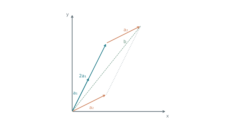
The product reveals two different ways of analysing this problem. Firstly, we can see the product as a linear combination of the columns of with weights , such that: When considering this system, the question we ask becomes: what combination of the columns of (the vectors , , ) yield the vector ? Our problem becomes finding a way to construct the vector from these columns. The columns of are the crux of its transformation, showing us where the standard basis vectors are transformed to by .
These columns span a subspace consisting of all their linear combinations, called the column space of . This column space is the output space of the transformation - every vector that is transformed by ends up in its column space. When we solve , we find , the coefficients telling us how to construct in terms of the basis of this column space.
The second way of analysing the problem is to look at the multiplication in terms of the rows of matrix . Each entry of is the dot product of one row of with , such that:
In this picture, every row of the matrix defines some constraint on the vector . Consider, as an example, the first dot product
This dot product establishes a constraint on , requiring that its elements must sum to two. Any whose elements do not sum to two will not be allowed as a solution to the system. We can see each row of as a linear functional of , taking an inner product with and acting as a linear map from to the scalar field . Each dot product is a new constraint on , requiring that the functional achieve a specific value. While the "column picture" looks at building the vector from components, this "row picture" tries to find the only vector that satisfies certain constraints.
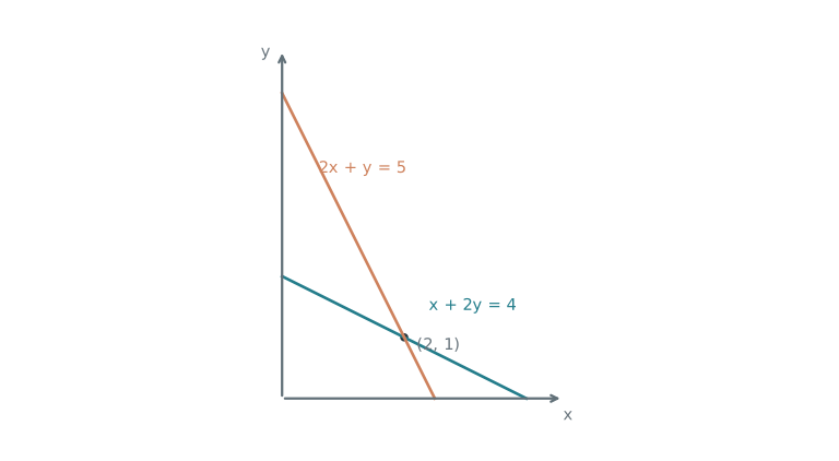
Each constraint defines an -dimensional subspace of , consisting of all vectors that satisfy the constraint. If we have independent rows in the matrix , we will have such subspaces. Our solution must lie at the intersection of all these subspaces, where all constraints are simultaneously satisfied. The diagram below shows two lines, each line is the set of points that satisfies one of the constraints. The solution to the system lies in their intersection.
The column space , is the output space of the transformation. A solution exists if and only if the vector is inside this column space. Then it can be expressed as a part of the output space, in terms of its bases (the independent columns of ). For uniqueness of a solution , there must be independent columns, such that has a unique representation in terms of those bases.
In the row picture, for there to be a unique solution, the intersection between the hyperplanes must be a single point. If the intersection is of higher dimension, there are an infinite number of solutions, since an infinite number of vectors satisfy all of the conditions. The row picture requires independent rows.
Linear Regression
Introduction to Least Squares
Consider the learning problem described earlier. We observe data points (where each is an input value and each is the observed output), and wish to find the line that fits these points best. We can express this as a series of linear equations:
We must remember, however, that we will almost never find the exact values of the unknowns and that satisfy this set of linear equations. In this example we have equations and only two unknowns. As a consequence the column space of the coefficient matrix , , lives in but is at most two dimensional. Our matrix is very long but not wide.
In general, we will have many more observations than unknowns, since collecting data is always easier than adding new observation parameters. Our observed data vector lives in the full -dimensional space whereas takes up only a very small portion of this space. Because is so vast in comparison to , even small experimental errors are sufficient to prevent the data vector from falling into this narrow column space, meaning there is no exact solution . A better formulation of the linear equations would be to write that we want to find a vector such that:
and is the best possible approximation. Just as with we did with earlier linear equations, we can represent our input data in a coefficient matrix , and vectors and . We consider then the product:
Since we want to find the best possible approximate solution, we need to formulate what it means to be the "best possible". To do this, we define a difference vector, often called the error . This is the difference between the observed result and our predicted result . We write this as:
Due to measurement error and the dimensions of the spaces, there will be no single line that passes perfectly through all points. Gaussian elimination, which relies on row operations to find a unique solution vector, will fail.
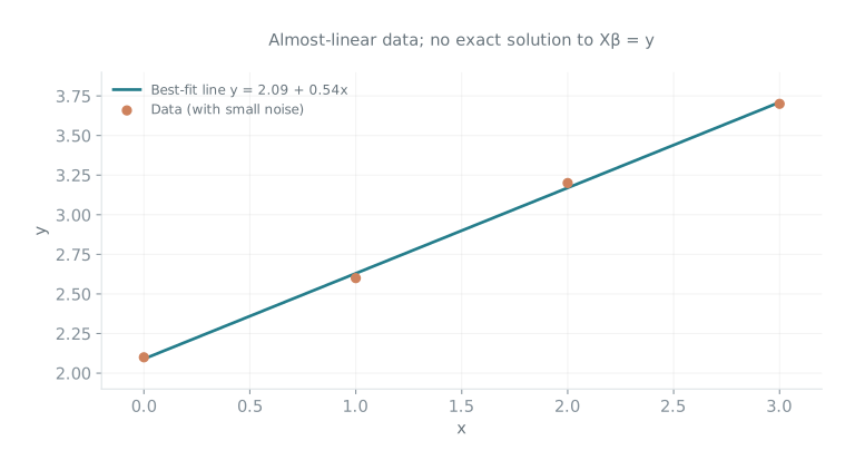
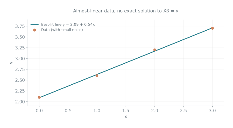
Consider four example measurements. They are each very close to a linear relationship, but each has small error such that it deviates slightly from the theoretical line: We can eagerly try to find a model by solving the linear system exactly, where To do this we form an augmented matrix and apply Gaussian elimination: The bottom rows assert that , or that , which is impossible. Gaussian elimination proves that the system is inconsistent and that the vector does not lie in the two-dimensional column space, . There is no exact solution. The graphical representation of these data points makes this clear. When we plot the theoretical line of best fit (which this chapter will work out how to derive), we see that no point lies precisely on this line - there is no straight line passes through all of these observations.
The solution to this problem lies in minimizing the error between what we can achieve (, which must lie in the column space of ) and what we desire ( which lies outside it). Since we cannot make exactly, we seek that makes as close as possible to .
The principle of least squares, introduced independently by Carl Friedrich Gauss who applied it to astronomical problems in 1795, and by Adrien-Marie Legendre in 1805, suggests minimizing the sum of squared errors. Then we can write: For each observation the term is our prediction, being the value our model assigned to . The residual is the error. Since the squared Euclidean norm of any vector is We can write that
The sum of squared errors represents an elegant link between geometry and algebra. It gives both the squared numerical error between our prediction and the actual value, and the squared distance between the point (our observations) and the point (our predictions) in -dimensional space. Minimizing means finding the values of and that make these two points as close as possible. Fundamentally, this minimisation problem represents finding the shortest path from our observations to the plane of possible predictions.
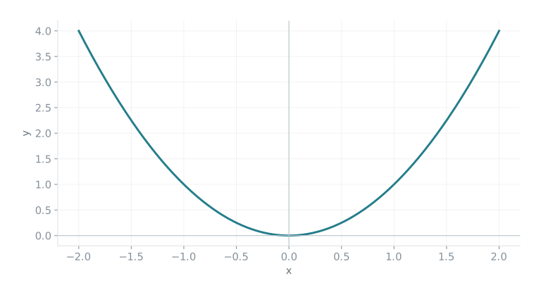
Beyond this, the choice of squared error is useful to us because of computational convenience. Consider, briefly, the unsquared error . As visible in the figure below, this function has a sharp corner at the point where the prediction equals the observation and we have zero error. At this point, the derivative jumps discontinuously from to , meaning the function is not differentiable at .
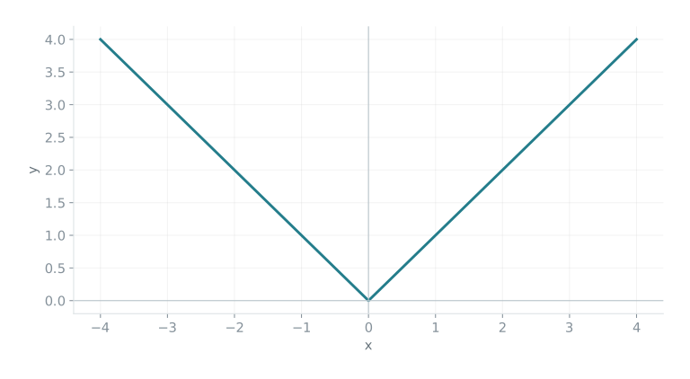
If we consider, as a contrast, the parabolic graph of squared error we see that it is differentiable everywhere.
Since the function is differentiable everywhere, we can take partial derivatives with respect to and , such that:
These derivatives exist everywhere and are continuous. Consider again the graph of the squared error parabola shown in the figure above. The minimum value of the parabola must come at a turning point, since that is where the function turns from moving down to moving up, and a parabola has one turning point only. This is obvious visually from the graph above. At a turning point, the partial derivatives are zero, so we can learn more about squared error’s turning point by setting the derivatives to zero:
: Dividing by yields: Equivalently: if we let be our predictions. Beautifully, these equations derived through relatively simple algebraic steps provide insight into what the ’best fit’ solution means. The first equation shows us that the sum of residuals must equal zero. This means geometrically that the residual errors balance out, such that we never systematically over- or under-predict. The line of best fit that we predict doesn’t consistently sit above or below the data points. The second equation shows us something more profound, demonstrating algebraically that the residuals are orthogonal to our feature vector . The summed product represents the inner product between and
A zero dot product is the condition for orthogonality. Since our design matrix has columns and , and it follows directly that:
meaning that each column of has a zero dot product with , or equivalently that is orthogonal to the whole column space .
More generally, this shows us the geometric essence of least squares. The core idea is to find such that is the point in closest to . As visible in the diagram below, the orthogonal projection of a vector onto a subspace is the unique point in such that the vector is orthogonal to .
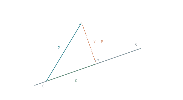
We can turn an algebraic problem into a geometric one. Since we derived that and , we can say that the point (where is the best fitted estimate), is the orthogonal projection of onto the column space. Then our residual vector represents the shortest path (shown as in the diagram above) from our observed data to its projection in the column space. This is the irreducable error that is orthogonal to the model space.
To minimize the residual must be perpendicular to the column space. The geometric principle is that the shortest path from a point to subspace is the perpendicular. We see this in -D, where the shortest distance from a point to a line is found by dropping the perpendicular. Projecting orthogonally onto a subspace in -dimensions is the learned approximation with minimal error.
Fascinatingly, from what began as an optimisation problem using calculus has revealed the fundamental geometric principle of least squares and linear regression as a whole, that the best approximate solution is always the geometric projection. This is the solution that minimises the length of the orthogonal , giving us the smallest distance between our prediction and the observed data. This is what corresponds to the minimum point on the quadratic from earlier.
The Normal Equations
Let us consider one more time the coefficient matrix and the response vector . We seek such that approximates . The smallest possible error must be the error directly orthogonal to the column space of , as we demonstrated in the last section, such that: Expanding this equation:
This represents the fundamental goal of least squares established at the beginning of this chapter. This is no longer an equation seeking a precise solution to , rather it is an equation that finds the that minimises . Since these equations are fundamentally based around the geometric base of orthogonality via , we call them the normal equations.
The matrix is always , since is , and the vector is . Then is a system of equations and unknowns. In general, if we have is , while before we would have had equations and unknowns for , we now have a system of equations and unknowns. This is a square system that can be solved using standard techniques such as Gaussian elimination.
To demonstrate this, we can show algebraically what the system of equations will look like. For our specific design matrix , we can compute . (I realise that most readers will prefer to gloss over the next few pages, those readers are excused and should feel no guilt in doing so. Please ensure, however, that you notice the highlights on pages 13 and 15.)
We compute :
The normal equations therefore become:
Expanding yields the system:
This is our final system of equations, which has two equations and two unknowns and . Since we have come this far already, the writer cannot resist going the extra step to solve for :
We solve this system of equations using Gaussian elimination. To eliminate from the second equation, we multiply the first equation by :
Subtracting this from the second equation:
Factorising:
Multiplying both sides by :
Applying back substitution, substituting this result into the first equation:
It turns out that there is a more elegant way in which one can rewrite these formulae for and in terms of the deviations from the means and .
Considering the numerator of , we can show that:
We now expand the right side:
Since :
The same applies to the denominator:
Hence we write that:
A fundamental beauty of algebra is highlighted in the simplification from the complex sums of page 14 to the significantly simpler and more elegant sums above. Geometrically, the algebraic steps represented centering the data, eliminating the complicated cross-terms that absolute positioning brings. For instance, the complex numerator transforms into the elegant centered form where each data point is now measured relative to the sample means rather than the arbitrary origin. The complexity in the original equations arose because everything was measured relative to an origin that had no relevance to our data. Centering sets the origin of our coordinate system at the center of mass of our data, revealing the true geometric relationships.
The final formulae for and are profound because they reveal algebraically some fundamental insights about the nature of learning. This is because the formulae can be expressed in terms of variance and covariance. Variance is a statistical measure of how much a variable spreads out from its average. Since we measure deviation from the mean using (where the square eliminates the negatives) for some , we can say that the variance of a variable is:
Covariance is a measure of of how two variables move together with respect to their means. If covariance is large and positive, then when is above its mean, tends to be above its mean too. And when is below its mean, tends to be below its mean too. They rise and fall together. We can write a formula for covariance, similarly as we did the formula for variance, as
Now consider again our original equations for and :
The denominator of our formula for is times the variance of and the numerator is times the covariance of and ! Our formula for is the ratio between the covariance of and and the variance of . This means we can write:
is the slope of the least squares solution. What we derived algebraically, that is covariance divided by variance gives us valuable information about the nature of the slope. Suppose our values were tightly clustered around their mean, with a low variance. Then even a small covariance between and would produce a steep slope, since we are dividing by a small variance. The - slope measures how much changes with a small change in . When has limited spread, even small changes in will result in large changes per unit , since we are dividing by a large variance. If our values are widely scattered with high variance, we need a much larger covariance to produce the same slope.
This scaling builds a bridge between the algebra and geometry of least squares. Algebraically, we take the covariance variance ratio, but geometrically, this has the effect of ensuring that measures the predictive relationship between and and also accounts for the natural variability present in the input variable. The learned slope is calibrated to both the scale and spread of our data.
The Projection Matrix
To wrap up our study of linear regressions, we can now generalise our specific least squares solution to the full matrix solution. If we consider the normal equations: Since , we can solve for the parameters , such that:
Matrices are so beautiful because of their versatility throughout mathematics. While they can be seen as just a simple table of numbers, they also represent transformations of space, systems of equations, the computational steps to solve the equations, geometric projections, and much more.
The matrix 1 accomplishes four things at once: it solves the normal equations , minimises the sum of squared errors , computes the geometric projection of onto the column space of , and finds the coefficients that extract the most information about the - relationship. Here, geometry, algebra and statistics converge.
Let us conclude this section with the example from earlier. We had four measurements that were very close to a straight line, but each had a small experimental error: We wanted to fit the model by solving the linear system exactly, but found that Gaussian elimination could not solve the system - was not in the column space of . We now have the tools to find the best approximate solution, the line of best fit.
To compute the inverse of , we find its determinant determinant , so Therefore: We have computed our linear regression, such that the line of best fit is therefore:
Deep Learning
Linear regression methods find the best linear approximation by solving . This fits the best possible linear surface to our data, such that computes the surface height of at point . Linear regression has one fundamental shortcoming: it confines us to the space of linear functions.
Consider the following problem2 We want a linear model that can map the following input tuples to their respective outputs: , , , . This problem is called the XOR problem. XOR stands for "exclusive or", where the "or" part means the output is true when one of the inputs is , and the exclusive part means that this excludes the case when both inputs are . This differs slightly from the problems we saw earlier with linear regression because it is a classification problem. While least squares methods give us the best linear prediction for a continuous target, here we want a linear classifier that will return either or , True or False. To reuse our linear machinery, we establish a score: and then classify by its sign, predicting True if and False if . This exposes the geometric perspective of the linear classifier, where the set is a hyperplane that divides space into two half-spaces. For all input points on one side of the hyperplane our model returns False; for all points on the other side it returns True. 3
A fundamental result of the 1960s was the discovery that no linear function can separate the classes from , , , . For this to happen, a linear model with weights and would have to satisfy: If the output of the model were positive we would assign one, if it were negative we would assign zero. A contradiction emerges when we sum the second and third inequalities: since we have . Subtracting from both sides of the last inequality gives: Then , which contradicts . This contradiction demonstrates that no linear model can separate the two classes, that is to say that no hyperplane can implement the XOR function on these four points. Figure 3.1 below shows visually why no decision boundary can divide the zeroes from the ones in XOR.
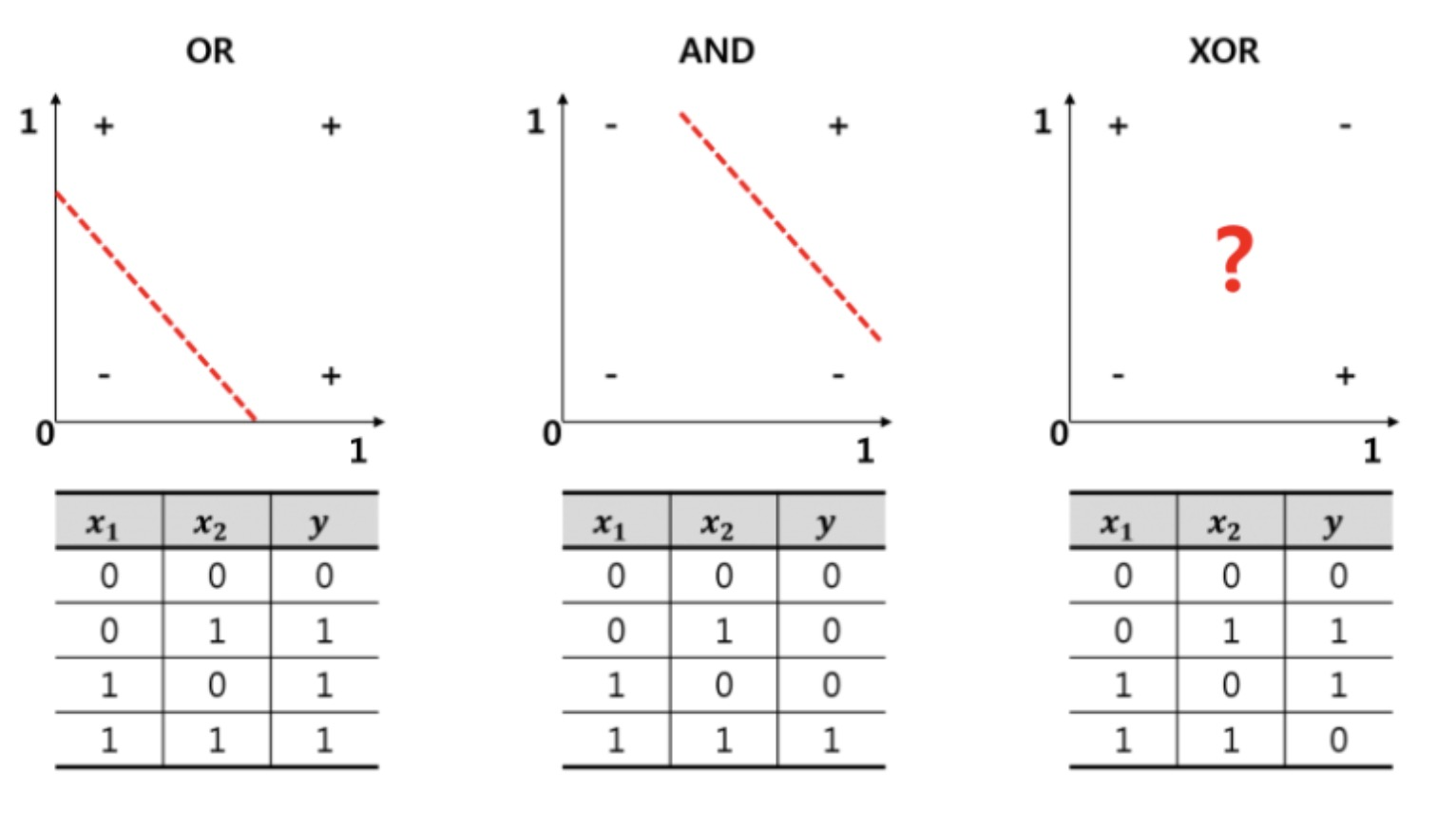
This demonstrates the fundamental principle of deep learning: to learn anything that contains nonlinearity, we need nonlinearity in our learning algorithm. XOR is fundamentally a nonlinear learning problem, since there is no way to draw a straight line separating the classes. Instead of a single linear transformation, we must compose multiple affine maps, each with nonlinearities. If we use a three layer network to learn our function, where each subsequent layer gets the outputs from the previous one, we can write this as where is some nonlinear activation function.
A famous result in the world of Deep Learning is Cybenko’s universal approximation theorem demonstrates that a network with a single hidden layer of sufficient width can approximate any continuous function on a bounded set to arbitrary precision. More precisely, for any continuous where is a bounded set, is our network, and any , there exist weights such that:
Moving from linear to composed models with nonlinearities means that we inevitably loose uniqueness of solution and must resort to iterative optimization with no guarantee of finding the optimum. The loss surface is filled with various saddle points and local minima.
What deep learning gains, however, is far better than this. Neural networks achieve generalisation. While linear regression worked only for linear relationships, neural networks have universal function approximation such that they can, in principle, learn to represent any continuous function to arbitrary precision. making them extraordinarily flexible learning machines. This is the power of deep learning with neural networks. It is the universal learning algorithm that can learn anything.
The Neuron
In 1837, Czech anatomist Jan Purkyně was examining thin slices of neural tissue, taken from the cerebellum. Purkyně discovered large, flask-shaped cells that were distinct from anything previously documented. The cells had a strange structure, with tree-like branches that extended in all directions. They were named the "Purkinje cells" and were postulated to represent the most basic nerve cells. Beyond this, however, the nervous system remained a mystery to scientists.
"A fundamental breakthrough came in 1873 when Italian physician Camillo Golgi, working in a home laboratory, discovered by accident that a solution of potassium dichromate and silver nitrate could stain individual neurons black. For the first time the full structure of these cells was visible. These cells were unlike anything anyone had ever seen before. Under the microscope emerged intricate cells with central bodies from which delicate, tree-like dendrites branched out on one side while long, thread-like axons extended from the other.
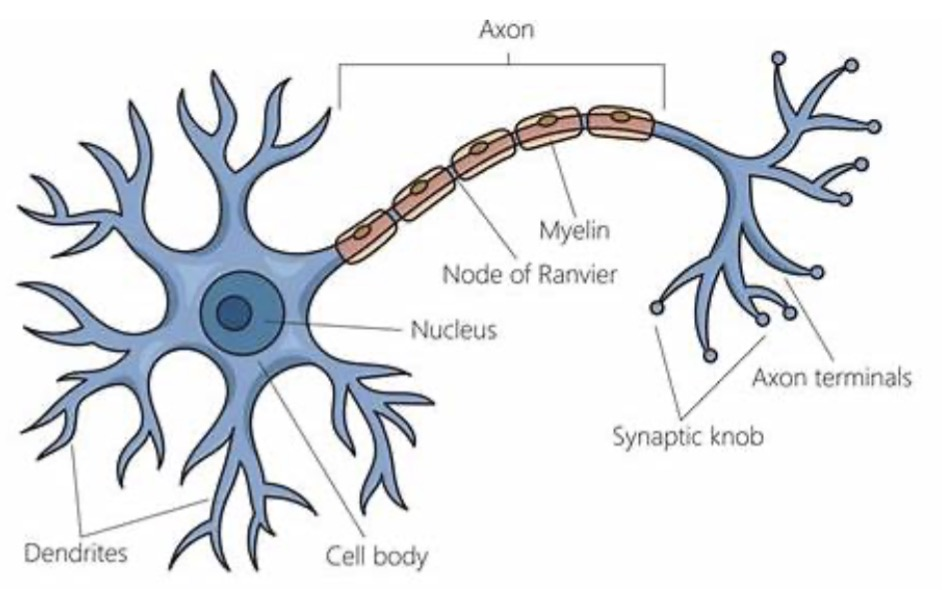
Golgi believed that these neurons were fused together in a continuous chain. Further study proved him false, instead they were found to be individual units that communicated across tiny gaps by electrical potential. These gaps were later called "synapses." Individual neurons were found to maintain a tiny voltage across their membranes, around -70 millivolts. When enough input signals arrived at the dendrites, the voltage would rise to a critical threshold of -55 millivolts which would trigger a rapid release of sodium ions. This would cause the voltage to spike to +40 millivolts, causing an electrical pulse, called the action potential, to travel down the axon to signal other neurons. The neuron has "fired".
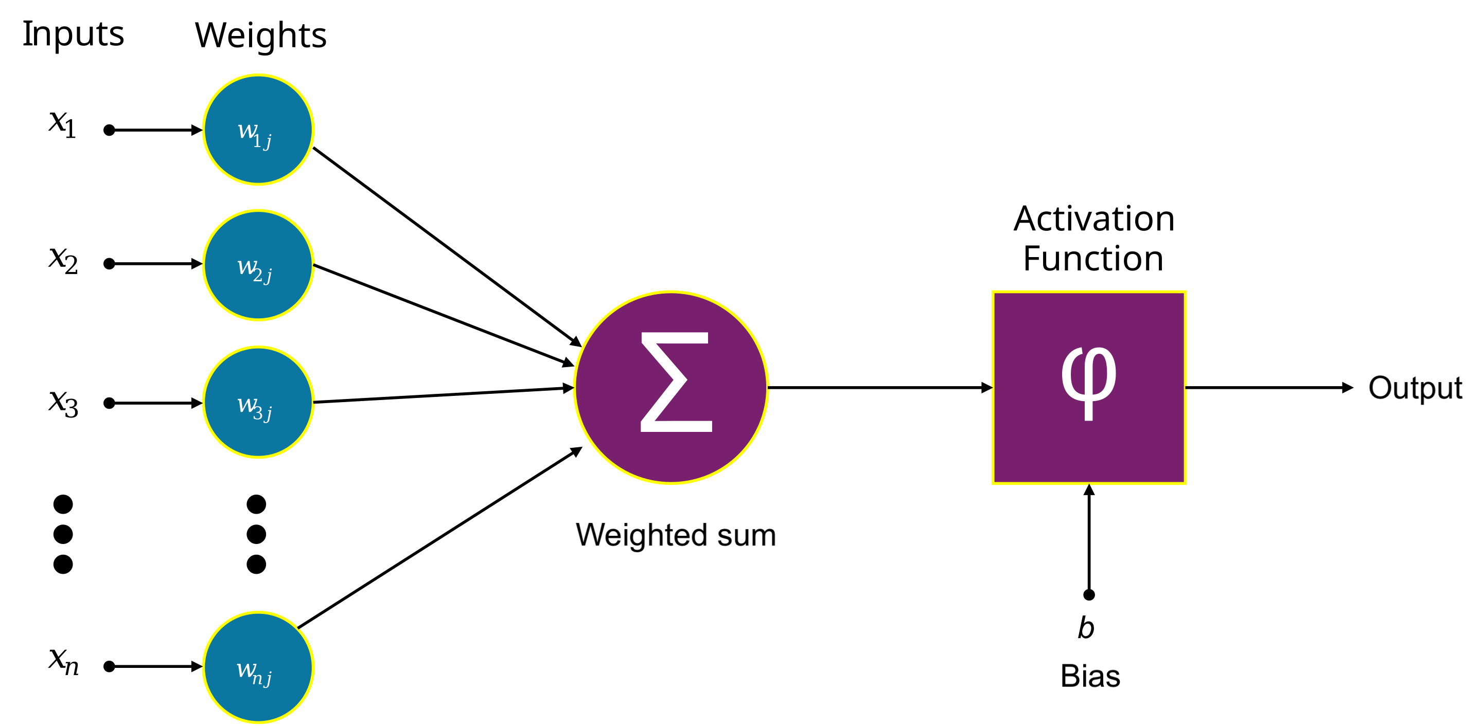
Although the biology of the nervous system is extraordinarily complex, neurons themselves are not too difficult to model mathematically. The neuron receives as input a series of voltages via the synapses. Each synapse has an efficacy (a measure of how well it transmits the charge). We can model this by assigning each connection a "synaptic strength". Each neuron weights its inputs by multiplying by a weight vector , where represents the synaptic strength of the connection with the th neuron. The input charges combine in the cell body, so in our artificial neuron the cell body is the sum of all . This is equivalent to taking the dot product between the vectors:
Biologically, every neuron has a different baseline activation level, such that some neurons are naturally more or less ready to fire. We model this in an artificial neuron by adding a bias to our sum, such that we have: With a large positive bias, the neuron fires with less input. Large negative bias raises the neuron’s natural inhibition and a greater input is needed to fire.
The neuron obeys a very binary firing pattern - either its threshold is reached and it fires, or its threshold isn’t reached, it doesn’t fire and the charge is dissipated. We model this through use of an activation function. This is a nonlinear function that determines the neuron’s final output to subsequent neurons based on the its aggregated input . A neuron with weights , bias and nonlinearity , given an -dimensional vector as input produces as an output
Figure 3.3 shows a schematic diagram of this process.
As we saw in the example of XOR, nonlinear activation functions are very important for neural networks. Linearity means the output for a sum of inputs equals the sum of the outputs. Most things don’t add - for instance images or patterns do not combine into new useful features by simple addition. They cannot be learned through linear methods alone.
Without nonlinearities, even the deepest networks would collapse to a single linear transformation. Consider a network with layers and no nonlinear activation function (such that each layer is just a matrix ): The product of two linear transformations is itself linear. No matter how many we stack, we can still learn linear functions only, and the whole premise of deep learning pointless.
To model the complex nonlinearity found in neurons, we use simplified continuous functions that are enough to capture the nonlinearity but are not overly complex. One such function often used is the hyperbolic tangent function: is continuous and differentiable everywhere. We can compute its derivative from the earlier expression:
Consider the graph of .
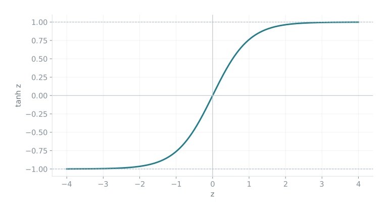
This graph highlights why is often used to model the nonlinearities in neurons. Firstly, for , . The artificial neuron using has a steep threshold such that it is almost always either "on" () or "off" (), just like the binary nature of action potentials in neurons.
The graph of also has a near linear region for small . Near , , the derivative . This has the convenient effect that small signals pass through unchanged. This is valuable to us because it means the neuron doesn’t muffle small signals which are often very important for later layers. At its core, performs a smooth squashing of space such that an infinite input range is compressed to finite outputs, but order is preserved, if , then .
In 2010, a new activation function, called the Rectified Linear Unit or ReLU for short, became popular. ReLU is defined as:
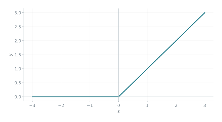
ReLU is a very simple function, outputting the input value for positive numbers and zero for negative numbers. Despite its simplicity, ReLU has several remarkable properties that make it highly effective for neural networks. For any given input, many ReLU neurons will output exactly zero, meaning only a subset of neurons remain active. This creates a sparse activation pattern that helps the network focus on the most relevant features for each input. When a ReLU neuron outputs zero, it effectively "turns off" that pathway, allowing the network to ignore irrelevant information and concentrate computational resources on useful signals. This selective activation mirrors biological neural networks, where only a small percentage of neurons (approximately 1-4%) are active at any given moment, creating efficient and focused information processing.
As we can see from its graph, ReLU has a simple derivative:
This means that for active neurons (), gradients flow through unchanged during backpropogation. Computing this derivative is also very computationally efficient. ReLU helps to mitigate the gradient vanishing problem that occurs when training deep networks, when during backpropagation through many layers gradients can become progressively smaller due to multiplication of small derivatives. Since ReLU’s derivative is one for active neurons, gradients can flow through these neurons without being dampened allowing for the training of deeper networks.
The Neural Network
A single artificial neuron computes: where: is the input vector, is a weight vector of learnable parameters, is a learnable bias term and is an activation function. Then is the output.
A layer of neurons is a parallel collection of neurons that operate in parallel. Each neuron in the layer receives the same input vector from the previous layer, where the th component of is the output from the th neuron in the previous layer. Each neuron then passes its output to every neuron in the next layer. The strength of each connection is determined by the weights in the receiving neurons’ weight vectors. If we have neurons in one layer, we can write the entire layer’s computation concisely with matrix notation:
If there are neurons in the current layer and neurons in the previous layer, then is the layer’s weight matrix, where each row in represents the weights for one neuron. The element represents the connection strength between the th neuron in the layer the th neuron in the previous layer. is the bias vector. is the nonlinearity. Note that is applied element-wise, such that . Finally is the layer’s output vector, and is passed on as input to the subsequent layer.
Each layer performs two operations. Firstly, it takes a weighted combination of the inputs using the synaptic strengths and adds the bias term. It computes an affine transformation, to yield . Secondly, it applies the nonlinear activation function element-wise to produce the output . .
The linear part applies some transformation on the input space. The nonlinear part ensures that every neuron adds something new to the network, preventing the network from collapsing to a single linear transformation. The standard notation for neural nets is to denote the -th layer’s weights as and its biases as . Then we can write a neural network as a composed function where .
We can use neural nets to correctly solve the XOR problem. As inputs we provide:
If represents the weight matrix of the th layer, and represents the bias of the th layer, we describe our network
We set our weights to:
The first layer’s weight matrix has identical rows . This means that both hidden neurons in the network compute the same linear combination + . Their different biases create distinct detection mechanisms. The first neuron computes , which activates whenever one neuron is positive, and the second neuron computes , which only activates when both neurons are positive (since is required for positive argument to ).
The second layer the detectors from the previous layer with weights to compute This implements the logical expression “at least one input active” minus “both inputs active”. The coefficient (rather than ) is crucial because when both inputs are active rather than , so we need to correctly output zero for the case. For the cases and we have yielding For both hidden units output zero, giving . Thus the network converts the linearly inseparable XOR pattern into a linearly separable one in the two-dimensional hidden space, where the final layer needs only a simple linear combination to distinguish the desired outputs.
Let . Then
We verify on the set :
Backpropagation
Modern artificial intelligence models, which are all based on neural networks have huge amounts of parameters. The parameters of a neural network are its learnable parts, consisting of its weights in the matrices and its biases . GPT-5 has approximately 600 billion parameters. As of September 2025, Meta’s Llama-4 "Behemoth" has the greatest number of parameters of any model, with a total of 2 billion parameters. Each parameter is a continuous value that is typically represented as a 32-bit floating-point number. If we consider GPT-5 again, the space of possible parameter configurations is therefore .
We could not possibly search this space for the best parameter configuration for our learning problem, since we have finite time and finite compute. GPT-5 was trained over a period of a few months using approximately FLOPS.
To do this, we need a good algorithm to train our model, updating the parameters (weights of the neural network) until we find the best parameters solve our problem or learn from our data. The algorithm we use to do this is called backpropagation, a remarkably simple application of the chain rule.
To measure how far away our prediction is from our expected result, we define a loss function . To update the parameters in our favour, we need a way that is better than brute-force to measure how much changing a specific parameter changes the final output. That is to say for a neural network with parameters and loss function , we need the gradient: Each component represents the change in the loss if parameter is incremented by .
The backpropagation algorithm comprises two steps: a forward pass and a backward pass. The forward pass computes the final value of an expression given inputs, and the backward pass implements the chain rule. If we know , we can compute:
. Consider the function with , .
We compute the forward pass
We then compute the backward pass (starting with ):
We can verify: , so and .
The core idea is that we can think of a neural network as a very complicated mathematical expression, and use backpropagation just as above.
Consider a simple 2-layer network with input , weights , , , : Then the forward pass computes: The backward pass computes gradients by reversing the graph and applying the chain rule at each node. Starting with : Propagating backwards through the graph.
We recall the chain rule such that if , then:
Neural networks obey a generalised form of the chain rule, where we look at total derivative. This is called the generalised chain rule. If variable influences loss through multiple paths via intermediate variables : This is why we accumulate gradients: each path from a parameter to the loss contributes additively to the parameter’s gradient.
The power of backpropogation does not lie in its capabilities, rather in its efficiency. We could compute derivatives alongside forward computation. For each input variable , we propagate forward through the graph. This is wildly inefficient as it requires one forward pass for each input parameter. This is computationally inefficient. It is a algorithm.
In backpropogation, we first do a forward pass to compute all values, then propagate gradients backward. For each output variable , we propagate backward through the graph. This requires one forward pass and one backward pass. It is complexity.
Once we have computed all of the gradients, we can update each parameter using an algorithm called gradient descent. The basic update rule is trivially simple: where is the learning rate, a small positive number (typically to ) that controls how big steps we take. The negative sign means we move in the direction opposite to the gradient, moving toward a lower loss.
In practice, modern neural network training uses significantly more sophisticated optimisers such as stochastic gradient descent, which uses individual examples to compute gradients, or Adam and AdamW that adapt the learning rate for each parameter individually and include momentum terms to smooth out the updates.
Broadly, however, the entire training process becomes to compute gradients via backpropagation, update all of the parameters simultaneously and finally repeat for thousands or millions of iterations until the loss converges at some value.
Networks Fold Space
If we want to understand what neural networks accomplish, we must abandon comfortable abstractions of "learning patterns" and "extracting features". Instead, we should confront the geometric reality that neural networks, and neurons themselves work by folding space.
Consider a single neuron with ReLU activation. It takes input vector and computes If we then consider the set: The point where is a very important one, because this is the boundary between ReLU activation - for all ReLU will activate, but for all , ReLU does not activate. Our set divides space into two half-spaces,
Since the boundary between and is the hyperplane , we can write that
Interestingly, when we examine more closely ReLU’s geometry, we see that it does not divide space in two but folds it in half. On one side of the hyperplane (in the half space ), ReLU collapses everything to zero, such that the entire half-space is crushed onto the hyperplane . On the other side, the space passes through linearly and its structure is maintained.
Let us explore the ReLU’s geometric implications on the space. If we consider the distance between two points before and after ReLU, after ReLU this distance becomes regardless of their original separation. Meanwhile, for : where is the angle between and . The distance is preserved, albeit under a projection
Instead of considering only a single neuron, let us now consider a whole layer of neurons. We compute . Each row of defines its own hyperplane, folding space into two:
For a layer of neurons, then, we compute:
Each neuron in the layer folds space according to its learned activation patterns in and . The hyperplanes partition into regions. An interested reader might ask themselves: how many regions (let this be) are created by hyperplanes in in -dimensional space?
Consider what happens when we add the th hyperplane to an arrangement of existing hyperplanes in space. This hyperplane intersects the existing arrangement, and then is divided into further regions by the intersections with the other hyperplanes. The number of regions on the new hyperplane equals , and each such region splits an existing region in two. Then Recursion with base cases and has been proven to yield the result: For , this gives us regions. For , we get
Each hyperplane separates space in such a way that on one side an individual neuron is activated and on the other it is not, each region represents a binary vector indicating which neurons are active and which neurons aren’t. Within each region, the layer implements a linear transformation: where contains only the rows of corresponding to active neurons (), with other rows zeroed.
Let us now consider a full neural network - a network of layers of neurons, where each layer takes as input the output of the previous layer. Then each layer takes the already folded space from the previous layer and folds it again. That is to say that the composition of layers creates a function : where each .
At the core of is the idea that the number of linear regions grows exponentially with depth. Each layer can potentially split every existing layer from the previous region, which leads to a multiplicative growth.
Each region created by the intersecting hyperplanes represents a distinct computational mode that the network learned during its training. Within any single region, the network applies a specific linear transformation. If we consider a region in space where neurons in set are active at layer , the transformation becomes: where contains only the rows of corresponding to active neurons (those in ), with inactive neurons contributing zero.
Across the entire network, within each region, complex composition that is multiple ReLU layers collapses into a single affine transformation: where and are the effective linear transformation and bias vector for that specific region. This is why neural network learning is not about the calculus we use in training but its linear algebra - a large neural network can learn things and generalise because it applies many linear transformations. Neural nets do not learn so well because they capture global nonlinearity, but rather because they learn to be locally linear everywhere.
This also explains the profound successes of Deep Learning. As we increase the depth of the network, this translates into exponentially more regions, which translates directly into exponential increases in learning capacity. More regions allow the network to make finer distinctions between inputs, enabling it to approximate increasingly complex functions with higher precision. A shallow network with few regions must use crude approximations, perhaps having only for one large region and for another. But a deep network with exponentially many regions can have thousands of precisely tuned linear transformations each of which is optimised for its specific slice of input space. In practice, training optimises each region for particular feature detection roles. Because of the hierarchical nature of folds in space, a deep network creates folds of folds, building complex decision boundaries through composition..
Universal approximation
The theoretical bedrock for neural networks is the Universal Approximation Theorem, first proved by George Cybenko in 1989. It claims that a network with just a single hidden layer, given enough neurons, can approximate any function to any desired degree of accuracy. Formally, the theorem states that given any continuous function on a bounded subset of and , there exists a network that can evaluate to within the accuracy. This network has the form: Then Cybenko’s theorem states that:
Consider a single neuron in this network. We first generalise the idea of activation function away from just and to say that the neuron will have a sigmoid-like activation function. A function is sigmoidal if
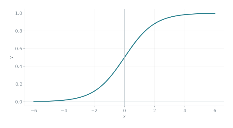
and the function is continuous and differentiable. Figure 3.6 below shows an example sigmoidal function. By Cybenko’s definition, is actually not sigmoidal since . However, follows the same sigmoidal shape and can be rescaled to get a sigmoidal function by Cybenko’s definition by writing . ReLU is not sigmoidal since it isn’t differentiable everywhere, however the limits match those of a sigmoidal. Both are sigmoid-like, so this is a pretty good generalisation for activation function. The most basic atom of the neural network is the single neuron, which computes .
The core part of this neuron is the linear computation . is a vector in high dimensional space, and is a measuring device, projecting down to a single number, . This equation geometrically defines a hyperplane, where is a vector perpendicular to the plane, defining the plane’s tilt. This is an affine subspace, and the vector defines how high the subspace is pushed up.
The result is passed through the sigmoid activation function . The sigmoid squashes the infinite range of into a finite range from to . The core decision boundary in space is where - for , the output is consistently near one. For , the output is consistently near zero. The transition between these states is a smooth shaped curve centered around the boundary .
This ramp can be made arbitrarily steep by scaling the input . Consider a scaled sigmod As the scaling factor , the ramp becomes vertical. Then we can write that:
where is the Heaviside step function defined as:
This limiting relationship is mathematically powerful because it lets us construct our proof using simple step functions that jump instantly from to , while we know that any such construction can be faithfully reproduced using sigmoid functions with sufficiently steep transitions, such that they can be easily translated back to the differentiable world of neural networks.
A single neuron gives us a step function that divides all of space into two regions. It outputs values near on one side of the hyperplane and values near on the other side. This is limiting for function approximation because it can only represent functions that are piecewise constant, with exactly two pieces separated by a single hyperplane.
For generalised functional approximation, we need something more localised, a function that is in a specific region and everywhere else. To manipulate neurons into creating this localised behavior, we can combine two neurons working in opposition. Consider two parallel hyperplanes defined by where . The first neuron activates when we cross the first plane, and the second neuron activates when we cross the second plane. By taking their difference, we construct a ridge function: This combination of neurons creates a function that equals in the controllable strip between the two parallel planes and everywhere else. We can now build a structure to use many such strips to approximate any continuous function .
To do this, we tile the entire domain with these strips. Each strip has its own height (controlled by the coefficient ). By adjusting the heights, the tiling produces a "staircase" approximation to our target function . If we consider again the ridge function from earlie, only with slightly different notation:
By inspection, when and equals everywhere else. We use this fact to build an approximating function: The function is constant within each strip, with value in the first strip, in the second strip, and so on, thus forming a step function that approximates .
Our domain is closed and bounded, is continuous on . As a consequence, is uniformly continuous on . Regular continuity means that moving a small distance causes only a small change in the function value. What counts as "small", however, could vary from location to location. Since the domain is closed and bounded our function cannot have arbitrarily steep sections because there isn’t infinite space available for curves with increasing slopes or infinitely long regions of steepness. Uniform continuity means that there exists a universal step size that works everywhere simultaneously, ensuring that the same small distance produces small function changes regardless of location in the domain.
We exploit the uniform continuity of the finite and bounded set to choose the widths and heights of our strips. Given desired accuracy , uniform continuity gives us a , representing the maximum width of a strip with the guarantee that the function variation within the strip is less than . We assign each function strip width exactly:
For each strip we choose the height . We do this simply by setting for some point in the -th strip.
If we have some , and some , w Any point falls into exactly one strip, say the -th strip. In that strip for some in the same strip. Since the strip width is , we have , and by uniform continuity
We should remember that this was demonstrated using the Heaviside functions and not the actual sigmoids. We can now replace each Heaviside function with a scaled sigmoid, recalling that: Our final neural network approximation is: With an arbitrarily steep sigmoid in our neural net approximation, we can do the same as we did with the Heaviside functions
Our final neural network approximation is:
With an arbitrarily steep sigmoid in our neural network approximation, we can achieve the same functional approximation as we did with the Heaviside functions. Each ridge function is constructed from two neurons working in opposition - the first neuron has weights and bias , computing . This creates a step that “turns on” at position . The second neuron has weights and bias . It computes , creating a step at . When we take their difference with coefficient , we get a function of neurons that equals between the two positions and zero elsewhere.
As , each scaled sigmoid approaches the corresponding step function . Since these functions are on a closed and bounded domain , all arguments to our sigmoid functions are bounded, allowing us to choose large enough so that everywhere on .
This construction achieves exactly what Cybenko’s theorem promises. Our approximating function has the standard neural network form: where each ridge contributes two neurons with appropriately chosen weights and biases, giving us a single-hidden-layer network with neurons.
The error analysis completes our proof: Since was arbitrary, we can obtain any desired accuracy by first choosing the strip width via uniform continuity and then selecting large enough to make the sigmoid approximation sufficiently steep. We have thus constructed a neural network of Cybenko’s required form that approximates any continuous function on a compact domain to any desired degree of accuracy.
This is called the Moore-Penrose pseudoinverse of , denoted . Regular matrix inverses only exist for square, invertible matrices, but the pseudoinverse extends this concept to any matrix. Its mathematical robustness makes the pseudoinverse a cornerstone of computational linear algebra and machine learning.↩︎
This problem was a famous problem during the ’early days’ of AI in the 1960s. Early AI focused on learning linear decision boundaries. A linear decision boundary is a straight line (or hyperplane) separator to separate "yes" outputs from "no" outputs. Just like least squares, this learning method could only model linear relationships. The XOR problem exposed a fundamental limitation of linear-based learning models (Minsky & Papert, 1969) and helped drive work on hidden layers and nonlinear features.↩︎
One can even find by least squares by setting labels to and using least squares to try and fit .↩︎