Approximation Theory
Approximation theory is the field of analysis that explores how to approximate things. It does this in the broadest sense - it deals with approximating functions, constants, distances, and providing algorithms to approximate anything that could be approximated. It is likely one of the most useful pieces of pure mathematics, applications ranging from approximating Einstein’s equations for relativity to constructing computer graphics using the Bézier curves formed by the Bernstein polynomials.
This project is divided is divided into three main chapters: one on functional analysis, one on the approximation of , and one on polynomial interpolation and its application to sequences.
The approximation of constants has existed since almost the dawn of mathematics, beginning to be necessary with the Greek and Indian discovery of the irrational following the Pythagorean theorem. However, the other fields of approximation theory are much more modern, the reason for this being that a precise notion and definition of a function is required for them, which was only first developed with the work of Bernoulli in the late 18th century.
Approximation theory then developed as a supposed solution to several problems, including Euler’s work on minimizing error on the maps of Russia in attempting converge the non Euclidian geometry of the Earth into a 2 dimensional rectangular map. Aproximation theory greatly simplified this process. A similar problem was investigated by Nash in the 1950s.
From this followed Chebyshev and Fourier’s work on the approximation of functions, culminating in the work of Bernstein in his proof of the Weierstrass approximation theorem, proving that any function can be approximated by a polynomial. Polynomial interpolation was first developed through the work of Newton in the late 17th century, and reached its culmination with the work of Lagrange in 1795.
Because approximation theory is so broad, it shows how mathematics has evolved, beginning with Archimedes’ geometric approximations, showing the development of calculus and Newton’s use of the ’divided difference’ as the derivative was developed, going through to Taylor series and integration.
Now if only it was still 2016, then we would have a square date today, since
Functional approximation
Introduction
Given a continuous function defined over the closed interval , how can we represent as another function such that the difference between the two functions is as small as possible? Can we construct a summation, or infinite series in terms of simple functions such that the resulting approximation is as close as possible to the target function? The theorem which proves that we can do this is known as the Weierstrass approximation theorem which states that given function defined over closed interval and , it is possible to construct polynomial such that , and therefore that any function can be approximated as closely as desired by a polynomial. The Fourier and Chebyshev series on which I will elaborate below use the method of infinite summation of easier functions to approximate more complicated functions, and have astoundingly fast convergence rate. Although the mathematics asserts that the perfect approximation is formed when the series is evaluated at infinity, if we wish to evaluate this in practice, we can truncate the series at a value , forming a compromise between computational energy and accuracy.
Fourier analysis
Fourier analysis is the approximation of an often complicated function using only the sums of the sine and cosine functions, proposed by French mathematician Joseph Fourier, who in his classic 1822 paper "The analytical study of heat" showed that decomposing more complex functions into simpler ones made it much easier to solve differential equations. Specifically, Fourier was trying to solve the heat equation, which had been one of the biggest problems of the time. However, by simplifying the functions in the differential equation to just the sinusoidal functions, whose differential properties were well understood, Fourier managed to solve the heat equation. This method has become known as ’solving by Fourier series’. To demonstrate how the Fourier series works, consider a basic sine wave:
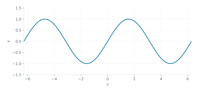
Now, consider the graph of :
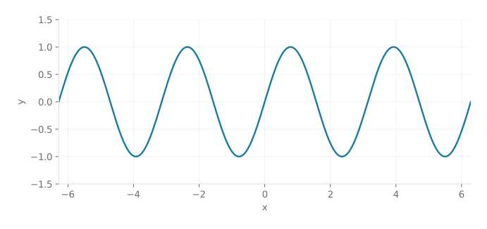
Now, consider this graph:
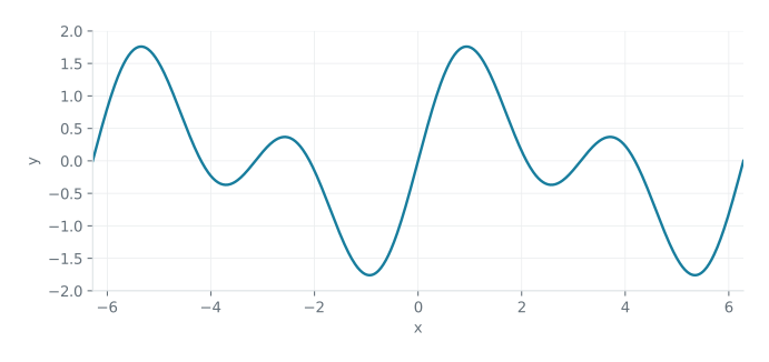
Note how dissimilar this graph is, on first examination, to the original two graphs. Given just this graph (and with no prior experience of Fourier analysis) you would assume that the graph is that of a strange and irregular function. However, this graph is just the graph of the function: This is the base for Fourier analysis. Given any function, how can we simplify it into just the sum of the sine and cosine functions?
This gives rise to two fields of approximation:
The Fourier series: Any continuous, differentiable oscillatory function can be (using the Fourier series) described as the sum of trigonometric or exponential functions. In order to ensure convergence, the Dirichlet conditions much be met - these being that the function must be periodic, absolutely integrable over its period, have a finite number of discontinuities and a finite number of maxima and minima.
The Fourier transform: Any continuous, differentiable function satisfying all the Dirichlet conditions except periodicity, can be described as a continuous integral of a complex exponential function.
Fourier Series
Let us first examine the Fourier series. What we want to achieve is an infinite series approximation for , in terms of the sine and cosine functions, weighted by index which has the effect of reducing the wavelength of the function and increasing accuracy and convergence of the approximation. We need to work out formulas for coefficients , and : In practice, when using the Fourier series to approximate a function, we will not evaluate the series to infinity, we will instead cut it off at a certain value of iterations, in a compromise between computational efficiency and convergence. Note that we do not need to have formula for .
Deriving the coefficients
How can we find and ? Recall first from linear algebra that one of the most basic operations which can be applied to two vectors is the dot product. We refer to the dot product as a dot in the middle of the multiplication (eg. ). Given two vectors , their dot product is given by either where is the length of vector and is the angle between the two vectors or: The first formula has quite an elegant geometric interpretation - consider, for the sake of example, two vectors and in 2 dimensional space.
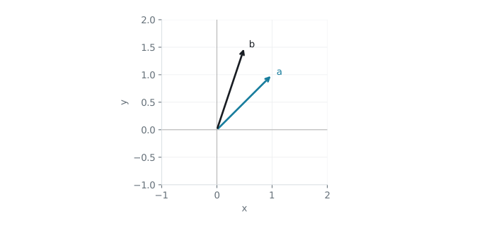
Consider the line formed by extending the line formed by connecting the tip of and the origin. The dot product is formed by projecting onto this line, and then multiplying the length of the projected by the length of , the result is the dot product of the two vectors. This is why the cosine teresting property of this is that this property does not change whether is being projected unto the line formed by or vise versa, both cases give the dot product. One more property of this dot product is that if the two vectors are orthogonal () the dot product evaluates to 0, whereas if they point in opposite directions, their dot product is negative. Let us furthermore consider how the second formula which states that if given two nth dimensional vectors, we can establish the dot product by simply summating the product of each element in both vectors (this will be of great use to us later) corresponds to the principle of projecting one vector unto another.
How can we apply this, to test whether two given functions and are orthogonal? We must represent our function as a vector, which we could do by forming a single row vector of infinitesimal increments, and then forming the dot product, which in the vector results in multiplying all the values in each row and summating this. This is essentially equivalent to the Riemann sum over and , therefore the dot product in the vector of our function is equal to
Where and are the ends of the function.
If we apply this to the trigonometric functions we are working with, we can take their dot product such that To evaluate this integral, we use the product-to-sum identity of the cosine function, which states that Our integral therefore simplifies to: Therefore, by the first Fundamental Theorem of Calculus, we can say that As the sine function crosses the axis for multiples of , will evaluate to 0, therefore, for , . For , both terms become: The integral of over any interval of is simply , while the integral of over a full period of evaluates to 0. Thus, when , Therefore: This means that multiples of cosine and are orthogonal in the dot product for and are in the dot product for . We consider whether this applies to the sine function by similarly taking we use the product-to-sum identities to simplify the integrand. The product-to-sum identities state that: Using this identity, we rewrite the integrand as: Now, we integrate term by term. Since the integral of the cosine function over a full period is zero, we have, by the First Fundamental Theorem of Calculus: and similarly, We can therefore state that, for all : When , the integral becomes: The integral of over any interval of is , while the integral of over a full period of evaluates to 0. Thus, when , Therefore, similarly to cosine, in the dot product, sine is orthogonal for all multiples and returns for , such that: We finally consider whether the dot product of and (weighted by and respectively) demonstrates an orthogonality between the sinusoidal functions over their period. We consider the integral: Using the product-to-sum identities, we rewrite the integrand as:
Thus, the integral becomes:
Evaluating each integral separately, by the first Fundamental Theorem of Calculus, we find:
This holds true for all and , including the case where .
Since both integrals evaluate to zero, we conclude: And therefore that, for all and , the functions and are orthogonal by the dot product
This is another reason why the sinusoidal functions were so useful to Fourier as he was solving the heat equation, as well as the fact that the differential properties of the individual functions are well understood, when they are multiplied we can also very easily simplify differential equations thus formed.
We can use this orthogonality principle to attempt to separate out and from our original approximation for : The integrals demonstrated earlier show that for all . When , we have: Therefore we have discovered a formula for , namely that: for . The key to finding is to realise that, to ensure that the Fourier series is accurate, we need to include a constant term that represents the average value of the function over one period. The average value of a function is given by
By integrating the function over its entire period the formula captures the total area under the curve of the function over one complete cycle. Dividing the integral by the length of the period scales the integral result to represent an average over the entire period. This normalization ensures that the average value is independent of the period’s length, focusing solely on the function’s behavior within one complete cycle. The result of this computation gives the average height of the function over one period. In graphical terms, if you were to draw the function’s graph over one period, the height of the rectangle whose area equals the integral would represent the average value of the function over that period. Therefore, we can say that:
To achieve coefficient , we multiply by and integrate, such that Similarly, using the orthogonality principle, the integral will cancel to 0, for all . When , we have: which yields We therefore have the complete Fourier series: Note that, by beginning index n a t 1 for both series, we add a separate formula for . Note also that this must be divided by two so that be distributed equally between sine and cosine.
An important thing to note whilst approximating a function using the Fourier series is which of the functions sine and cosine should be used. Given an even function (where ) we use just the even cosine function, whereas given an odd function (where ) we use just the odd sine function. In all other cases we use both.
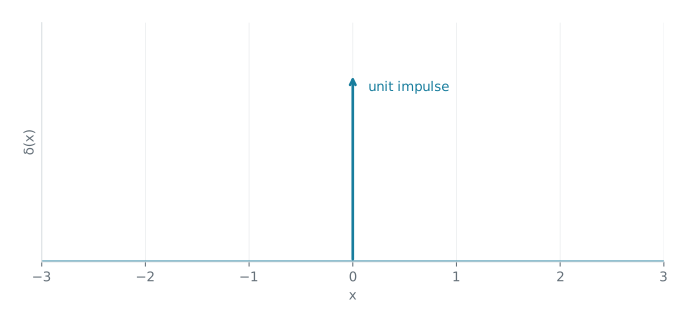 Diagram reconstructed for this web edition; original image not supplied.
Dirac Delta Function
Let us now use an example to illustrate the use of the Fourier series, namely the Dirac delta function. The Dirac delta function, denoted by , is shown in Figure 1.1 above. The Dirac delta function is very interesting, because it is equal to zero at all values except at . This function is very good for describing oscillatory behaviour - for example in an article I recently wrote for the most recent Axiom edition, I described how the periodic synchronization of fireflies can be modelled by showing that the probability of all fireflies flashing at time time must converge to the Dirac delta function.
We can loosely define this function as
However, this piecewise definition is not very elegant. It is better to define the delta function in terms of its properties - namely that Note that this function is even, therefore when using the Fourier series to approximate it we will not use sines, and only cosines. Therefore, if we approximate the delta function between and , we have: We also have the previously derived formula for We also know from the earlier given property that the integral of the delta function is always equal to one. Therefore: Now let us also evaluate . We can again use the previously named property. Furthermore, we must remember that the delta function returns 0 at all values except x = 0, therefore it isn’t really necessary for us to evaluate the integral as the multiplication will go to zero at all points except x = 0. In other words - in the multiplication, x = 0 is the only point which is interesting enough to consider. This point is very convenient as cos(0) = 1. Therefore, This formula for the constant tells us something amazing and very specific to the Dirac delta function - the constants remain constant regardless of . All the frequencies are the same. Normally, we would see a decay in values a , however, the singular delta function has constant coefficients throughout. The Fourier series for the Dirac delta function is therefore:
Complex Fourier exponential series
It is important for the sake of the Fourier transform which follows, that our series can be rewritten in terms of only a complex coefficient . We can do this because, if we have the set of complex exponentials where , we can say that these represent the base of the sine and cosine functions, where is the frequency of the wave. This is encapsulated by Euler’s formula that Euler’s formula is a beautiful mathematical identity that relates the exponential function, sine function, and cosine function in a single equation:
This formula is quite elegant because it combines these fundamental mathematical functions in a concise and profound way. This formula is derived using power series expansions. It can be shown that the exponential function can be represented as a power series:
Furthermore, the sine function can also be represented as a power series:
Similarly, the cosine function can be represented as a power series:
Now, let’s consider the expression :
Simplify each term:
Now, let’s group the real and imaginary parts:
Notice now that the real part is exactly the power series expansion of , and the imaginary part is exactly the power series expansion of . Thus, we have:
This formula can be made even more beautiful if we let , yielding which beautifully combines all the fundamental mathematical constants. Euler’s formula neatly represents the link between the exponential and sinusoidal functions, showing that we can rewrite our approimation in terms of just a complex coefficient and the exponential function. Therefore, we can approximate as Furthermore, shares a similar orthogonality principle with the sinusoidal functions. This can be shown by evaluating To solvce this, we can use Euler’s formula, derived earlier by the power series. We express and by Euler’s formula:
Substituting these expressions into the integral, we get:
Expanding this expression, we get:
Now, since is an even function and is an odd function, the integrals involving products of and over a symmetric interval like will all evaluate to zero. So we are left with:
Using the orthogonality property of sine and cosine functions, which states that:
and similarly for , we can evaluate the remaining integrals:
So, the integral becomes:
where is the Kronecker delta, defined as:
Therefore,
Demonstrating that, similar to the sinusoidal functions, the exponential functions are orthogonal by the dot product with different weights and for , whereas for , the dot product returns 0. Using this, we can derive the complex coefficient , by multiplying the equation by and integrating over the closed interval to yield Therefore, for all the integral is 0. When , it simplifies to , therefore we can write that From this, we can say that We can therefore write the complex exponential form of the Fourier series as
Fourier Transform
We will use the complex form of the Fourier series, which I wrote to be If we extrapolate from the sinusoidal functions with base period into an arbitrary (must satisfy all the Dirichlet conditions except that of periodicity) function of period , the whole formula can be rewritten in terms of the period L as: If we let where L is the interval on which we set the function. Now, in order to be able to take the Fourier transform, we want to know what happens when we take the limit This means we no longer will be considering a fixed period, but the entire real numbers. We can try to make the equations slightly less convoluted by defining It is important to note that when we summate these s over the ends of the function (being + and - infinity) what we are essentially doing is creating a grid in the axis with interval We define function Using this, we can rewrite our complex coefficient to be Therefore, the Fourier exponential series with becomes: Notice, however, that . Therefore: which is a much more aesthetic (and for our purposes useful) form. Recall that a Riemann sum approximates the integral of a function as the areas of a set of rectangles of equal width under a curve as the number of rectangles tends to infinity (or conversely the width of the rectangles tends to 0). It is written as:
where is the width of each subinterval, and represents the value of the function at a particular point within each subinterval (this can be done in terms of left endpoint, right endpoint and centrepoint sums, being in what way the rectangle is aligned with the curve, however for our purposes we deal only with the left endpoint Riemann sum). The similarity between our summation and the Riemann sum should now become visible - consider what happens as L approaches infinity in our previous summation: We know that will go to zero. Therefore, will go to 1. Recall the grid image I described earlier - as goes to 0, the grid will become infinitely dense. We can take out the to yield Now, if goes to zero (which it does), the Riemann sum can be made equivalent to the integral by saying that for Which extends the Fourier series across the entire real number line.
Chebyshev Approximation
A method of approximation came to the great Russian mathematician P. L. Chebyshev whilst he was working on the problem of linkages, specifically relating to translating the linear motion of steam engines to the circular motion of wheels. Linkages are devices composed of rigid bodies (called links) connected by joints or pivots. The problem of linkages more generally is that of converting any geometry of motion into any other geometry, which must not necessarily be linear. The problem is still greatly applicable today, examples of its application being in robotics, prosthetics and linkage based engines (which is the problem Chebyshev was working on), and research is still in progress, examples of papers including https://doi.org/10.48550/arXiv.1312.1060 (An algebraic study of linkages with helical joints, Abban et al., 2024) and https://doi.org/10.48550/arXiv.2307.13839 (Geometry of integrable linkages, Perline and Tabachnikov, 2023). Chebyshev is often called the father of Russian mathematics, a claim which is particularly backed up by his founding of the St. Petersburg Mathematical School, kickstarting Russian mathematics.
Pascal’s triangle and Chebyshev polynomials
Pascal’s triangle is formed by beginning with 1 at the top, and summing each number with the number next to it (imagining the triangle is in a space of infinite zeroes) forming the triangular array of the binomial coefficients arising in probability theory, combinatorics, and algebra. The beginning of the triangle is shown above as Figure 1.2. Pascal’s triangle is intrinsically linked to the Fibonacci numbers, a sequence defined inductively as: and with the first few terms being:
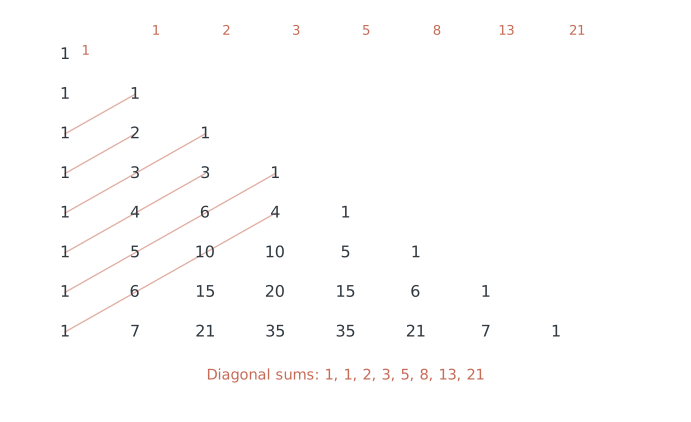 Diagram reconstructed for this web edition; original image not supplied.
Figure 1.2 also shows red lines, travelling in a northeast pattern and each time travelling down one place and to the right two from the previous index of the numbers. The numbers on the red line are then summated, resulting in the Fibonacci sequence. From these lines, we find the coefficients of an interesting set of polynomials: the Fibonacci polynomials. These are polynomials which use the same recursion as the Fibonacci numbers, and add a variable. They are defined as: We can therefore write out the first few Fibonacci polynomials as: Notice that the coefficients of the Fibonacci polynomial are simply the numbers along the red line. We can play around with Pascal’s triangle by changing the signs in every second diagonal.
From this, we can form a new set of polynomials: the Chebyshev polynomials of the second kind. These are formed in a very similar way as we formed the Fibonacci polynomials: this definition being identical to the one of Fibonacci polynomials, save that we changed the sign from a + to a - in the expression . As well as the Chebyshev polynomials of the second kind, Chebyshev also introduced the Chebyshev polynomials of the first kind, which are the polynomials which uniquely satisfy conditions The Chebyshev,polynomials of the first kind are also highly useful for approximation, but we will focus here on the second kind. Here the coefficient operate in the same way, being the same diagonal lines on the triangle as formed before (unfortunately LaTeX does not allow me to format the lines on a non-figure). Given this method of computing them, we can consider the first few Chebyshev polynomials and their graph below:
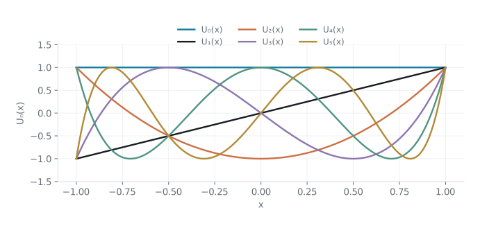
This graph is neat (a lot more so than that of the Fibonacci polynomials), and shows one of the fundamental properties of the Chebyshev polynomials, which will be of use to us later: they have very neat and roots.
Using the Chebyshev polynomials for approximation
These Chebyshev polynomials are extremely useful for approximation. This section will concern itself only with the Chebyshev polynomials of the second kind. What is important about them is that they minimize oscillations that can occur at the edges of the interval when using polynomial approximations. This is why, when Chebyshev polynomials are used for approximations, they are commonly only used between the interval [-1, 1]. The reason that the interval [-1, 1] is perfect for the use of Chebyshev polynomials is because Chebyshev polynomials have exactly real roots evenly (due to the symmmetry of about the origin) spaced out (as is visible in the graph above). Therefore, on the interval [-1, 1], function can be represented as Similarly as in the previous section on Fourier analysis, we need to derive . We will again, as in the section on Fourier analysis, need to exploit the property of orthogonality. Recall that two functions are orthogonal if and we let be the weight function (which we have previously just kept as 1). Now consider whether this is true in the case of the Chebyshev polynomials. Consider The Chebyshev polynomials are constructed in such a way that they are orthogonal with respect to weight function over the interval . Therefore, we can write that:
And for , which yields (with respect to ): Having now demonstrated that the Chebyshev polynomials are orthogonal, we can now levy this property by multiplying our previous expression by another Chebyshev polynomial . Therefore We can integrate over [-1, 1] so that Since we have discovered the behaviour of the integral of the multiple of two Chebyshev polynomials, we can say that the integral is 0, except when , Since we know that we can say that Therefore, we divide by the respective constant to yield: And Note that we need to multiply these constants by the weight function discussed earlier, in order to ensure the integral of the inner product can be correctly calculated with the orthogonality. Therefore: and
Approximation of
Mathematics is filled with beautiful and important irrational constants. This chapter will concern itself with just . is one of the most fundamental constants in all of mathematics (and I think the only mathematical object to which one of the 365 days of the year is dedicated) - it is the ratio formed by the geometric length of a locus of points equidistant with radius from a centrepoint, and the length . It is therefore the ratio between the diameter and the circumference of a circle. Hence comes the formula for the circumference This value was first proposed by Archimedes. However, how can we approximate it? How do we know it needs to be approximated and is not just rational?
Hermite’s proof that is irrational
A key question in the consideration of whether or not a constant can be approximated to complete accuracy is the question of whether or not it is irrational. This question was first considered by Johann Heinrich Lambert in the 1760s, who proved that is irrational, that is to say it cannot be described by a proper fraction. Lambert demonstrated this (although I will not go into the particulars here) by showing that this continued fraction expansion holds:
Then Lambert proved that if is non-zero and rational, then this expression must be irrational. However, , therefore is irrational, and so, therefore, is .
However, in the 19th century Charles Hermite created a much simpler proof, relying only on elementary calculus, such as that taught in the last few years of secondary schools today. Simplicity of ideas used is key in the development of fundamental proofs, and I think that Hermite’s proof demonstrates this beautifully. Hermite’s proof is now the most commonly used and taught proof for ’s irrationality.
Hermite’s proof operates through use of Reductio ad Absurdem, one of the most powerful techniques of proof by contradiction. It’s power was put perfectly by mathematician GH Hardy in his book A Mathematician’s Apology: "a chess player may offer the sacrifice of a pawn or even a piece, but a mathematician offers the game." (many thanks to NA for gifting me said book.) Let us first assume that can be expressed by a fraction: The next step of the proof is to define a sequence. This sequence is very interesting - its terms are as follows:
I realise that at first, resulting out of such simple terms and we have such an immensely complicated term , however the explanation for the formula is remarkably simple, and the resulting consequences are immense. Let us begin by attempting to evaluate the integral . Consider the function being integrated, defined over the interval [0, ] with variable positive values for n. The graphs all look relatively similar to this one (where n = 0.5):
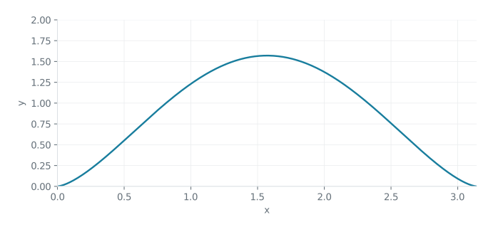
Note the fact that the curve begins at 0, comes up to a maximum value and then goes down to 0 again. Let us now consider the maximum possible value for the function, to get a rough idea for the area of the curve. Since we know that the factor in the integral cannot be greater than , achieved when . The second term is similarly equal to , however this is achieved when . Furthermore, can be at most 1. Therefore, when we take into account the entire function which is being integrated, we can definitively say that: Therefore, the maximum value for the function must be below the line . From this we can extend that the area must be less than the area formed by the lines and , and . Therefore, Simplification yields that: We now consider what happens when . Let us primarily consider the fraction , if we let , we are left with the more general problem - to what value will tend as ? As we now that factorial growth is greater than exponential growth, it is demonstrated that it will, in fact converge to 0. Therefore, it follows that sequence This is a fundamental step in the proof that is irrational. Recall that we begun with the assumption that can be described as a fraction , where and are positive integers. We have now demonstrated that the sequence converges to 0, if we can prove that this sequence is also made up of only positive integers based on the assumption that and are positive integers, we will have an absurdity - positive integers cannot converge to 0! Therefore we will have proved that and cannot be positive integers, proving that is irrational. In order to establish the fact that all integers in are positive integers, we need to create a recurrence relation for , based on and .
The proof that all values of the sequence lies in a way of rewriting this sequence as an inductive sequence. Earlier, I stated the first to values of the sequence I as and
Let me quickly demonstrate that these are true. The first is just the result of the simple and easy to evaluate integral The second term is slightly more difficult to derive, it comes from the integral This simplifies to This simplified integral simplifies to two much simpler, standard integrals for integration by parts, which simplifies the integral further to which simplifies to
Now we have fully established the starting values of the sequence, let us again use integration by parts to establish a recurrence relation. Let us evaluate the integral on a specific case in the sequence, namely that for . Consider the integral We can simplify this to: Note the interesting property that the formula looks very similar to what we established as the nth term, only the exponents are down by one, sine is replaced with cosine and we have some extra terms at the start. Let us now integrate by parts again, resulting in Some basic algebra simplifies this to This presents important progress, because the above expression can be split into two separate integrals, resulting in
This looks quite neatly simplified so far, so let’s now input it into our general formula for : This gives us one final step of simplification, resulting in This results in our proof. We can now simply replace with , and with . Off the back of this, we can build an inductive sequence, We can now make use of our assumption that pi is rational: Also note that . If we wanted to generalise this, we could write that Note that this does not prove the relation for all . In order to prove this for all , we can begin by considering the sequences of real functions:
We can inductively prove that these functions can be represented as infinite series, such that and therefore that From this, we can say that (using the quotient rule for differentiation) This is equivalent to saying that Notice an inherent similarity between this recurrence relation and the one which was demonstrated for - the final step in the proof is the idea that we can demonstrate that and are essentially the same function.
Therefore, given that base cases for the induction and are both integers, given further that the formula given for does not in any way change an input from integer form, we can safely say that any value in the sequence , resting on the assumption that can be expressed as a rational fraction . However, we have also demonstrated that as n approaches infinity, approaches 0. Integers cannot approach 0, as the closest they can be to 0 is 1. Therefore, we have demonstrated that our assumption that can be displayed as a rational fraction leads to an absurdity. Therefore, is irrational.
Archimedes’ approximations
Archimedes was working with circles when he first discovered a constant , which was to be the ratio between the diameter of a circle and its circumference. Therefore, Archimedes equated that . Consider first a square, with diameter d and perimeter . Therefore, if we take the ratio between the circumference and the diameter, we can say that, as a circle with same diameter can be fit inside a square, Now consider a regular hexagon, constructed in such a way that from each side to the centrepoint an equilateral triangle is formed. Therefore, if we let the sidelength of one of the equilateral triangles be , we know that the diameter of the hexagon is and its perimeter . Therefore, the ratio between the perimeter and diameter of this hexagon is 3. However, a circle with the same diameter as a hexagon can only be fit on the outside of the hexagon, therefore: We have now reduced the possible values for from the infinite set of real numbers to the infinite set of real numbers between 3 and 4, which represents progress nonetheless. However, Archimedes approximated even closer to its real value.
He did this by imagining a circle with diameter 1. He also knew that the circumference of this circle is . In our previous approximation, we used a hexago n and a square to approximate that is between 3 and 4. Consider what would happen if we replaced the square with a hexagon, thus having a hexagon circumscribed about a circle, as well as a circle circumscribed about a hexagon. We can divide the hexagon into equilateral triangles, each of sidelength the same as that of the hexagon. Therefore, using our previous numerical example, each edge of the inner hexagon is 0.5, therefore the inner perimeter is 3. On the outer triangle, we can do the same thing, however instead of knowing the sidelength of the triangle, we only know its height to be 0.5. We can split the triangle in half, resulting in a 30 60 90 triangle, which has the property that the ratio between the sides is . Therefore, the total outside perimeter is . We can therefore say that This gives us one method to approximate pi - we need a method to calculate the perimeter of a polygon with an arbitrary number of sides. To do this, we can use some basic trigonometry, however we must ensure not to use any results which already contain so as not to base our approximation on knowledge Archimedes would not have had. Let the perimeter of the circumscribed polygon be and the perimeter of the inscribed polygon be . Consider again a circle, with centre O of radius 0.5. Consider furthermore, a point A on the circumference of the circle, which is also the midpoint of a side of the polygon, and a point B on the edge between the same side of the circumscribed polygon as A, and the adjacent side. Let angle AôB be . Therefore, by the basic trigonometric ratios in which Archimedes would have been versed,
Furthermore, we can say that And that therefore the perimeter of the n-agon is simply We can follow a similar procedure with the inscribed polygon: let O be the centre of the circle, B the midpoint of one of the sides of the polygon, and A the vertex between the side on which A lies and an adjacent side. Therefore, we can again say that and furthermore that This is the formula Archimedes used to show that:
Ramanujan, Leibniz and Gregory’s approximation
Ramanujan was the son of a clerk in India, and despite not having had any training in mathematics, he came to publish some of the most important results in modern mathematics. Ramanujan was invited to Cambridge by G.H. Hardy, and it was during his time at Cambridge that he discovered his formula for . It is worth noting that Ramanujan derived many approximations for (see the Ramanujan-Sato series or Ramanujan’s modular equation), however I have chosen his series which is based on the arctangent function and adaptations to the Leibniz-Gregory series..
Ramanujan began by considering the arctangent series. This series is generally attributed to the work of James Gregory and Gottfried Leibniz in the 1670s. Consider the derivative of the arctangent function Now consider what happens if we take the indefinite integral of both sides As the integral of the derivative is simply equal to the original function, We now use the Taylor series approximation for this function. The Taylor series approximation of a function uses the derivative of this function at point to approximate it around . The Taylor series expansion of a function about a point is given by:
Alternatively, it can be expressed in sigma notation as:
If we consider the Taylor series expansion of a function about a point is given by:
In this case, . We find the derivatives of at to obtain the coefficients of the series.
Therefore the Taylor series expansion of about is:
We can insert this into our original formula: Let us now evaluate the integral of each term of the series. This results in
Consider now the case when :
Recall that Therefore, we multiply by 4 to obtain an approximation of :
This series converges slowly, so it may take many terms to get an accurate approximation of . This was one of the main problems Ramanujan saw with it, this slow convergence is what he sought to improve with his formula for . Ramanujan began with the formula that has been outlined above, and added a factor of . Ramanujan then ingeniously added the factor . His formula was therefore: Ramanujan’s minor changes to the formula make a massive difference. I run a python code and display its results in Table 2.1 to demonstrate this (for clarity the code has been included as Appendix 1 of this chapter). Note how big the differences remain (as a fraction of the individual differences), and that they are always on the same order of magnitude as , even when the value becomes
| Max term | |||
| 1 | 0.0623 | 0.4749 | 0.4125 |
| 2 | 0.0145 | 0.3250 | 0.3104 |
| 3 | 0.0037 | 0.2463 | 0.2426 |
| 4 | 0.0010 | 0.1980 | 0.1970 |
| 100 | 8.881784197001252e-16 | 0.009900747481198291 | 0.009900747481197403 |
| Computer cannot calculate low value | 9.999899927226608e-06 | Cannot be calculated |
Let us now try to understand why adding just these few simple factors has such a great effect. Consider first the addition of the factor . As increases, the factor exponentially decays as the denominator exponentially grows. This means that, as n approaches infinity, the increments become smaller and smaller, which means that oscillations around the true value are avoided, and the value approaches the true value as quickly as possible. The reason why Ramanujan’s additional factor avoids oscillations touches on the effect created by the the term inside the series . This term means that consecutive values of the series cancel each other out, however, if each term is not reduced quickly enough, major oscillations will form around the true value of . Minimizing the change in increment to a specific value means that the oscillations become succedingly less, as is demonstrated by the figure above. Furthermore multiplying by makes the series a geometric series. This is useful, because geometric series are easy to analyze, and it is easier to prove that they converge. Furthermore, describing the series as a geometric series provides a neat geometric interpretation of the terms, which represent lengths of line segments. This interpretation helps visualize the approximation process and understand how the series constructs an approximation of the circumference of a circle, and I will explore it later in this section. However, on a deeper note, I would argue that Ramanujan’s use of a geometric series reflects his mathematical intuition and creativity. By recognizing the series as a geometric progression, he was able to exploit its convergence properties to derive an elegant and efficient approximation for . In addition to this, Ramanujan added an additional factor of to the outside of the summation, which scales the series up by scaling each individual term The effect of this is to scale the series neatly up to precisely . The use of is interesting, and adds to the mystery surrounding the approximation and much of Ramanujan’s work - Ramanujan was famous for not including proofs or any real explenations for his results (until Hardy forced him to). The inclusion of adds an elegance through ’s geometric significance - below are just a few examples of its significance:
The ratio of the length of the side of an equilateral triangle to its altitude (the line segment from any vertex perpendicular to the opposite side) is . This ratio remains constant for all equilateral triangles.
Hexagonal patterns appear frequently in nature due to their efficient use of space. The square root of 3 is intimately related to the geometry of hexagons (which follows from the properties of equilateral triangles, as the shapes are closely linked). For instance, in a regular hexagon, the ratio of the length of a side to the length of the apothem (the distance from the center of the hexagon to the midpoint of a side) is .
The square root of 3 frequently appears in trigonometric calculations, especially involving the sine and cosine of certain angles. For example, in a 30-60-90 triangle, where one angle is 30 degrees and another is 60 degrees, the sine and cosine of 30 degrees are and respectively.
Furthermore, is irrational. However, it again cannot be denied that really, due to Ramanujan’s way of dreaming up new results, that this amazingly quick convergion of the series adds to the mystique, and beauty, surrounding Ramanujan’s work.
Code to evaluate and compare approximations for
import math

def ramanujan_series(n):
    pi_estimate = 0
    for i in range(n + 1):
        pi_estimate += ((-1) ** i) / ((2 * i + 1) * 3 ** i)
    pi_estimate *= 2 * math.sqrt(3)
    return pi_estimate

def original_series(n):
    pi_estimate = 0
    for i in range(n + 1):
        pi_estimate += ((-1) ** i) / (2 * i + 1)
    pi_estimate *= 4
    return pi_estimate

def true_pi():
    return math.pi

def calculate_error(n):
    pi_estimate_ramanujan = ramanujan_series(n)
    pi_estimate_original = original_series(n)
    pi_true = true_pi()
    error_ramanujan = abs(pi_estimate_ramanujan - pi_true)
    error_original = abs(pi_estimate_original - pi_true)

    return error_ramanujan, error_original

def main():
    n = int(input("Enter the index for the term in Ramanujan's series: "))
    error_ramanujan, error_original = calculate_error(n)
    print(f"Error using Ramanujan's formula at index {n}: {error_ramanujan}")
    print(f"Error using original formula at index {n}: {error_original}")
    print(f"Difference in errors: {abs(error_ramanujan - error_original)}")

main()
Polynomial interpolation
Introduction
The idea of interpolation follows on from the idea of functional approximation in that our aim is to define a function, as simple as possible, around a set of points, rather than simplify an existing function. In such a way, we can think of approximation as interpolation with infinite, rather than a finite number of points. This section explains interpolation through the lens of finding the term of an arbitrary sequence.
I define the term as the function that returns, given any integer less than or equal to the length of the sequence, the number in the sequence at index . There is a function which returns given any sequence . Therefore if: we can define , and . In this paper I explain several methods to return , culminating in a Python code which, given a sequence of any length, will return its term. Note however that, given only values of sequence, it is impossible to predict the next term as there are infinite curves which can go through a set of points with infinite possible values at the next value. This paper however focuses on finding the lowest order polynomial curve which passes through the points.
Interpolation by simultaneous equations
The term of sequences can be solved for by forming simultaneous equations in the form . Let each value of sequence be described by an coordinate in the plane, where the value is the index of the value in the sequence. We thus have: There is a line, which can pass through all the given points. Furthermore, this line can be a polynomial, as any number of any points may define a polynomial curve (see Appendix 1 for a proof). As it is a curve, its equation can be represented as an degree polynomial: We can thus substitute values for and and solve the equations simultaneously for , , , and , from which we receive the equation of the term. Let us illustrate this through an example. We thus have the cubic equation: Which can be solved by substituting values of and . This yields: We now have the general equation: Let us now insert : which correctly solves to:
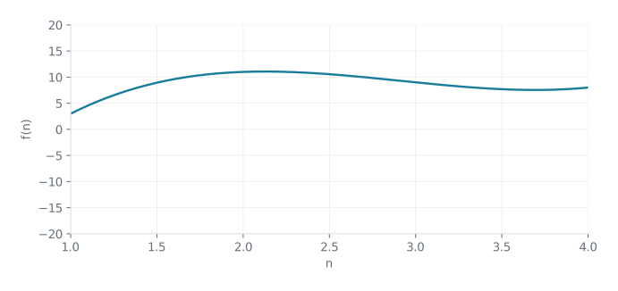
Although this is huge progress and presents a method for a human (or computer running standard methods such as elimination or substitution) to solve for the term of any sequence, the solution is an inefficient one. It finds the solution by brute force instead of using an elegant method. This solution works perfectly well when our sequence contains only three values, however the obvious question to ask when assessing such a solution is how it will work with a thousand, or a million values in the sequence. I am certain that I am not alone in thinking that solving 1000 simultaneous equations is neither an appealing nor elegant nor efficient solution to the problem. We have thus established a base in solving the problem, but we must now progress into more elegant and efficient solutions.
Lagrange Interpolation
For the sake of example, let there be 4 nodes. We can create a set of polynomials , , , and . To reduce oscillation and allow for scaling, these are based of the Kroenecker’s delta function. These polynomials are known as the Lagrange polynomials.
We can therefore say that the Lagrange interpolant over points can be written as: Where is the Lagrange polynomial at , and is the value at . We can loosely define Note that here is the point in where it is equal to the node, and represents any other node. This is essentially equivalent to Kroenecker’s delta function, which is a function which takes as input two variables and returns 1 if they are equal, and 0 if they are not.
It is not difficult for us to construct polynomial equal to zero at the points we want it to be - consider the polynomial: We know that this polynomial will be equal to 0 when or or . Let’s use this idea to make when we want it to. Say we have the nodes at , , and . Note for later the importance of this chronological order as we must remember that in most sequences, we will be given values in chronological order at indices 1, 2, 3 ... We want and , per our definition.
We can now make a "guess" of our Lagrange polynomial : Notice that this is precisely the same form as our prior polynomial equation except that , , and .
We can draw its graph, and notice that it equals 0 at the correct places, but at is equal to 2 instead of 1 per our earlier definition.
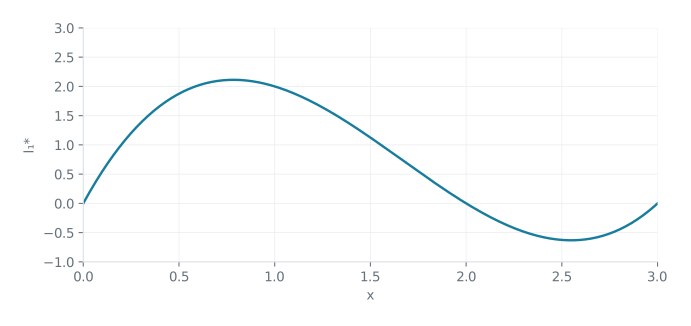
What can we do to fix this? Let us see what happens at : We have: 0 divided by any number is still 0, but any number divided by itself is equal to 1. We now have the correct formula, the graph of which is shown below:
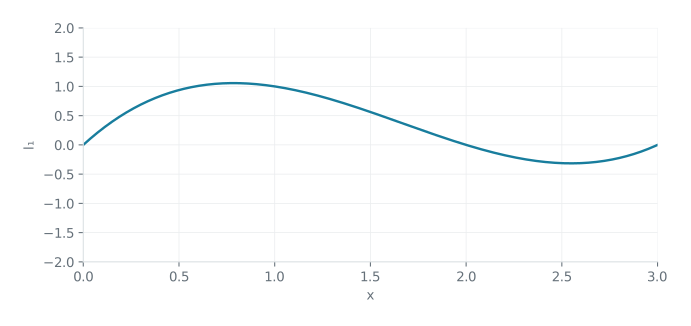
However, we have not fully defined the Lagrange polynomial for all values . We can formalise what we said earlier by saying that, given a set of nodes , you will have Lagrange polynomials such that the Lagrange polynomial is the product from to (excluding ) of divided by , into which the values for and can be substituted, forming a polynomial of degree per the formula below and the graph above:
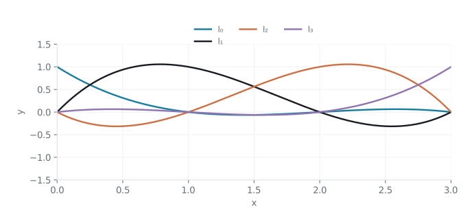
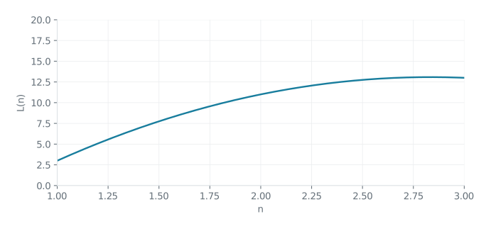
We can illustrate this through one example: Say we wish to find the term of the sequence (3, 11, 13). We can now establish the data points (1, 3), (2, 11), (3, 13). Then, we use the Lagrange interpolation formula to summate we get the following: We need to find out the value of , so per our earlier formula we can derive: Substituting our value for into the Lagrange interpolation formula we have: This simplifies to: Which is the term of the sequence as shown in the graph below.
Newtonian interpolation
We have again made huge progress on the efficiency scale, but there is still a big problem. The Lagrange method requires a huge amount of computational complexity, and is difficult to implement especially with higher order polynomials, due to the large amount of computations which must be done. This is nowhere as complex as solving 1000 simultaneous equations, but the algebraic simplifications and multiplications I did to achieve the formula for would be extremely complicated and slow for a machine to achieve. On the other hand, Lagrange’s method provides a very elegant solution (as I prove in Appendix 3). Perhaps, however, there is an equally elegant, but more computationally efficient and involving less calculations. The same question was asked and answered by Sir Isaac Newton, one of the most influential mathematicians and physicists of his time, known amongst many things for his inverse square law of gravity and his contributions to calculus.
Suppose you have the set of data points:
These values, as earlier discussed represent values of a certain function , which we must find. To do this, Newton uses divided differences. Divided differences can be understood as the change in the coordinates of two points divided by the change in the coordinate between the same two points. Thus, the divided difference is the average rate of change between the given points
This difference is a first-order divided difference. We now continue to calculate higher-order divided differences. Note however also the second part of the definition of the divided difference to provide a base case for recursion: We can now attempt to solve the problem. We can now continue calculating these divided differences recursively, using the last value for until we reach the maximum number of divided differences allowed by the data points, which is (for a set of points of size ) divided differences.
As a small aside - this plays in beautifully into calculus and taking the derivative (which is probably how Newton thought of it). When we take the derivative, we use almost exactly the same formula:
Visibly, the s in the denominator cancel. Perhaps the similarity is not immediately obvious, however remember that just refers to the value, we can thus think of as . Note that this is essentially the same as just taking the divided difference of and , which is often referred to in textbooks as the difference quotient. As we take the derivative, we want the instantaneous change, so thus the change as approaches 0. Therefore:
Returning to our prior equations - we can now generalise the example, for any size of dataset, to:
This generalisation links the recursive divided differences demonstrated earlier with a basis polynomial of degree , which is similar in nature by that used in the Lagrange polynomials.
We have now come to the final step - we summate all of these basis polynomials weighted by their respective divided difference, to ensure each of them contributes to the overall polynomial.
Say, as an example, we have the sequence:
This can be translated into the data points:
Therefore we can calculate the divided differences such that:
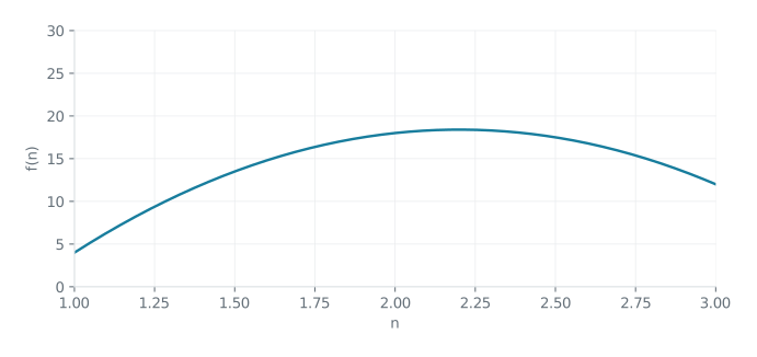
This is the polynomial term of the sequence, as is visible in the graph below:
We have now got three relatively competent methods of finding the term of any sequence and, more broadly, approximating a polynomial curve to any set of points. The method of simultaneous equations becomes extremely inefficient extremely quickly, however has the advantage that it is very intuitive and does not require a great deal of additional knowledge to implement. The Lagrange solution is slower in large datasets, however is arguably the fastest if the size of the dataset is known, (recall that in sequences we are given value in increasing chronological order ie at , , etc.) and we can then store the equations of various Lagrange interpolants at different nodes, which are then scaled achieve a specific value. The Newtonian solution is best for large data sets due to the neat use of recursion, and the simplicity of the calculations.
The appendices of this chapter follow on the next page.
Appendix 1: Lines through points
How can we prove that a method such as the Lagrange polynomial method will work for any set of points? First, we must prove that, given any number of any points, we can draw a polynomial curve through them. We know that to define a straight line (which is just a first degree polynomial) we require 2 points, to define a quadratic we require 3 points, to define a cubic we require 4 points etc. How can we prove that for any polynomial of degree can be defined by or more points. Given any set of distinct points where the -values are distinct, there exists a unique polynomial of degree passing through all these points.
We can denote the polynomial as . We need to find such that for all to .
We can set up simultaneous equations:
This gives us a system of linear equations with unknowns . Since the -values are distinct, the system of equations is non-singular, meaning it has a unique solution.
Therefore, there exists a unique polynomial of degree passing through all the given points. This applies to all points, and therefore any points can be described by a polynomial of degree .
Appendix 2: Calculating the efficiency of the various algorithms
To do this, we will use big O notation, a method of approximating the runtime of an algorithm by considering what happens as the size of the dataset/input grows arbitrarily large. This is a sister function to the little o notation, which compares the runtimes of different algorithms. The mathematical basis for Big O and little o notations were both developed by Paul Bachman and Edmund Landau, who (by interesting coincidence) happens to be my great uncle.
Efficiency of using simultaneous equations
: Calculating the efficiency of solving such simultaneous equations is tricky, as solving simultaneous equations depends very much on the equations themselves. However, for the purpose of finding efficiency, we will in some sense assume the worst - that the dataset is so bad that we must use generic methods such as elimination, which affect all the equations and thus the entire dataset. In big O notation, these result in . We can further explore this by attempting to understand what we do in the elimination method - we choose one equation as a pivot equation and use it to eliminate a certain variable from all other equations. We then repeat this for all equations. Thinking in terms of writing code: this involves two nested loops over rows and columns, resulting in a runtime of . However, the worst case scenario for the runtime of each row is therefore combined runtime is
Efficiency of Lagrange method
In the Lagrange method, we can go through similar logic as we did with the simultaneous equations: in the Lagrange method we evaluate the Lagrange polynomials at each point and then sum them after weighting them to appropriate values. Evaluating a Lagrange polynomial requires operations, and these must each be summed n times to give . However, if we had the polynomials stored for integer nodes, the efficiency would be , which would make it the most efficient algorithm.
Efficiency of Newton’s method
Again we can think this through in a similar way - calculating the divided differences table requires operations, we add this to the number of operations needed to separately evaluate the polynomial which are . However, in the equation the term dominates as increases - thus the efficiency of Newton’s method is
The Ultimatum: A code which will, given any sequence of integers return its term
The code:
from sympy import symbols
from fractions import Fraction

def calculate_divided_differences(indices, sequence_values, n):
    differences = [[Fraction(value) for value in sequence_values]]
    for j in range(1, n):
        differences.append([])
        for i in range(n - j):
            d = (differences[j - 1][i + 1] - differences[j - 1][i]) / (indices[i + j] - indices[i])
            differences[j].append(d)
    return differences

def interpolate(indices, sequence_values, n):
    differences = calculate_divided_differences(indices, sequence_values, n)
    term = symbols('n')
    polynomial = differences[0][0]
    x_term = 1

    for i in range(1, n):
        x_term *= (term - indices[i - 1])
        polynomial += differences[i][0] * x_term

    polynomial_str = str(polynomial).replace("**", "^").replace("*", "")

    return polynomial_str

sequence = [0, 0, 0, 0, 0, 0 , 0, 1]


indices = [i for i in range(len(sequence))]
n = len(sequence)

polynomial = interpolate(indices, sequence, n)
print("Nth term:", polynomial)
About my code: a walkthrough
:
1. General stats
This code takes input (as can be adjusted at the end of the code in the sequence values) a sequence of any number of values, and returns as output its term. Per my testings the code can do 10 values (each less than 10) in 0.2 seconds, 50 values in 0.6s, 100 values 1.2 seconds, and 1000 values (thank the random number generator I coded) in 39.2 seconds.
2. CalculateDividedDifferences function
Note that I have used capitals to indicate underscores as LaTeX doesn’t allow me to write them. This function takes as input three values: the list of sequence values as provided by the user, the list of indices (ie just counting [0, 1, 2...]) and the length of the sequence . Note that the only reason this function takes the indices and as input is due to the fact that the same values are needed in the next function - it is therefore more efficient to calculate them once and have the functions take them as input than to calculate them twice. We then initialize our list of differences, making use of the Fractions function from the fractions module to ensure that our calculations are neatly formatted at the end. We then loop over 1 to n, initialize a new row in the differences table and then iterate over a nested loop, which goes over the range from 0 to (note the is necessary when counting from 0.) We can now populate the table per Newton’s formula: I rewrite the recursion algorithm implicitly as a nested loop to reduce stack overflow.
Interpolate function
(Note that the same applies with underscores) The interpolate function takes as inputs the same arguments as the CalculateDividedDifferences functions - indices, SequenceValues and n. This function then runs the CalculateDividedDifferences function to create a 2d list differences. We then create a symbolic variable term of size n (it must be symbolic so that we an use the sympy library to manipulate it). We then initialise the polynomial to the first divided difference, which is the value of the function at the first point. We then initialise the xterm variable (which we will use to accumulate terms) to 1. We can now loop over 1 and n and multiply xterm by the difference between the current value of term and the previous index. We now add this to the polynomial variable, format nicely and return the polynomial.
Another code using the Lagrange method
from sympy import symbols, factor

def simplify_and_factorize(expression):
    factored_expression = factor(expression)
    factored_expression_str = str(factored_expression).replace("**", "^").replace("*", "")
    return factored_expression_str

def lagrange_interpolation(sequence):
    n = symbols('n')
    result = 0
    for i, term in enumerate(sequence):
        numerator = 1
        denominator = 1
        for j, other_term in enumerate(sequence):
            if i != j:
                numerator *= (n - j)
                denominator *= (i - j)
        result += term * numerator / denominator
    interpolated_expression = simplify_and_factorize(result)
    return interpolated_expression


sequence = [0, 0, 0, 0, 0, 0, 0, 1]

nth_term_expression = lagrange_interpolation(sequence)
print("The nth term of the sequence is:", nth_term_expression)